Basic Module Transfers, Movements, and Connections

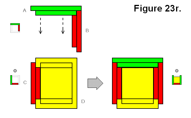
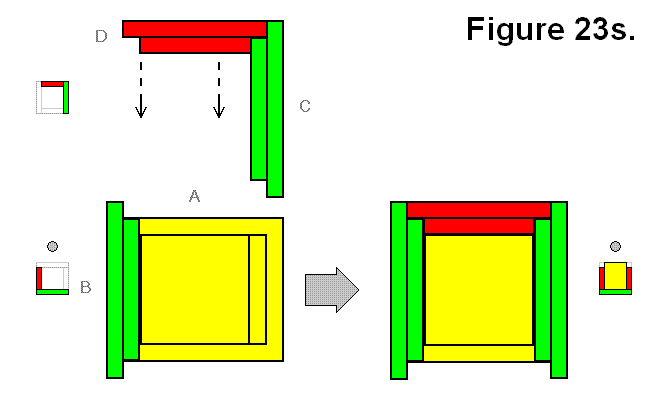
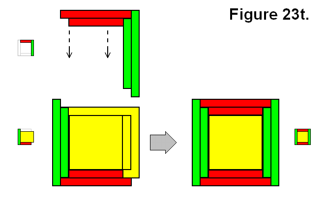
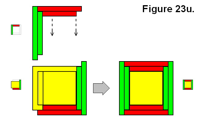
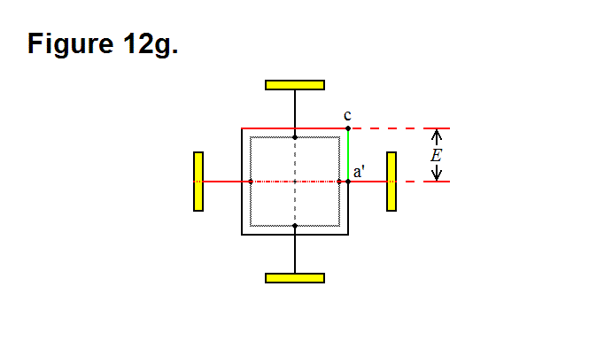
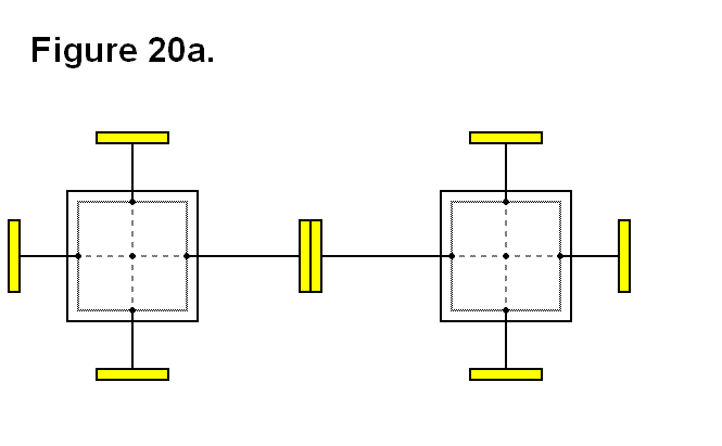
BASIC MODULE TRANSFERS, MOVEMENTS, AND CONNECTIONS

A module can be transferred around in a matrix of modules by pivoting and telescoping the legs, and connecting and disconnecting with the connecting plates. In Figure 4a, below, modules A-E are connected together to form a two dimensional matrix; in this matrix, module A is initially positioned in row 1, column 2, and its bottom leg connects to the top leg of module C, positioned in row 2, column 2. Module C is connected to and supported by the rest of the modules in the matrix through its bottom, left, and right legs. In the following figures, the legs for module A are drawn in different colors to illustrate their location in the movement as the module progresses from one position to another.

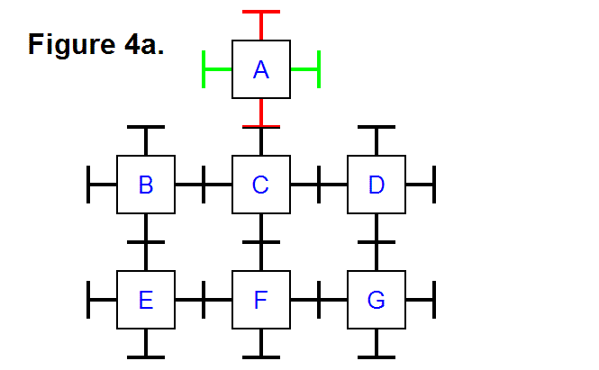
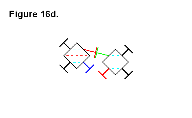
It is possible to transfer module A from row 1, column 2 to row 1, column 3, along the top surface of the rest of the matrix. Figure 4b, below, shows the same modules in Figure 4a, except that module A has been tilted by pivoting its bottom leg and the top leg of module C. The leg to the right of module A and the top leg of module D have also pivoted so the plates on the legs of these modules can connect to each other. The legs that pivot can also be extended so the connecting modules can reach each other, if necessary.

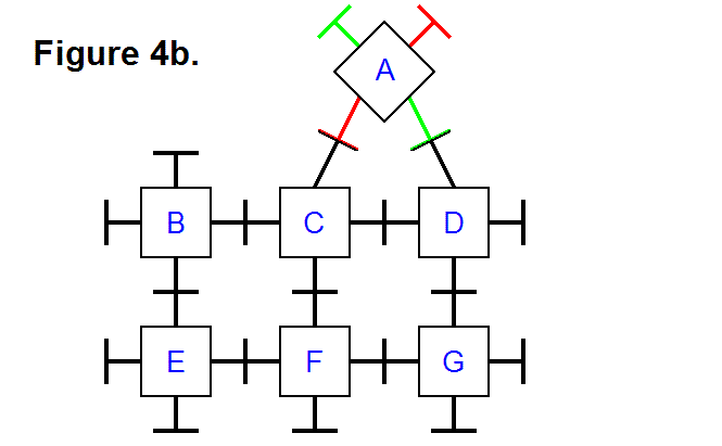
By reversing the motion of moving module A with module C and connecting it to module D, that is, disconnecting module A from module C and pivoting it upright with module D, module A is now in row 1, column 3; this is shown in Figure 4c, below.

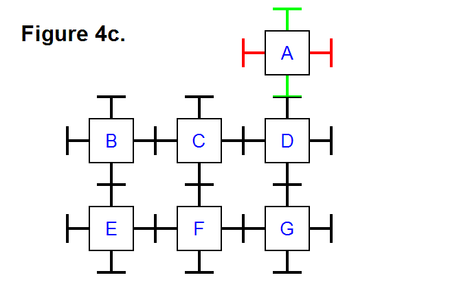
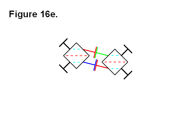
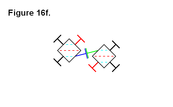
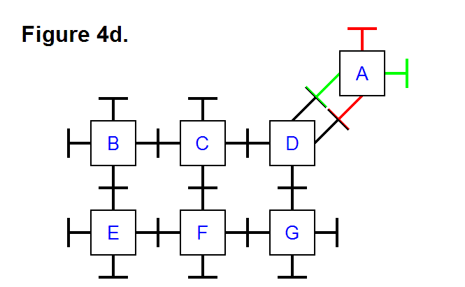
It is also possible to pivot a module around a corner of the matrix, such as with module A around module D from its top to its right side (position row 1, column 3 to position row 2, column 4). Figure 4d, below, shows the legs that connect modules A and D (the top leg of module D and the bottom leg of module A from Figure 4c) pivoted to allow the right leg of module D to pivot and connect to the bottom leg of module A (the same leg that was on the right side of module A in Figure 4c.), which was also pivoted into position for connecting to the leg from module D.

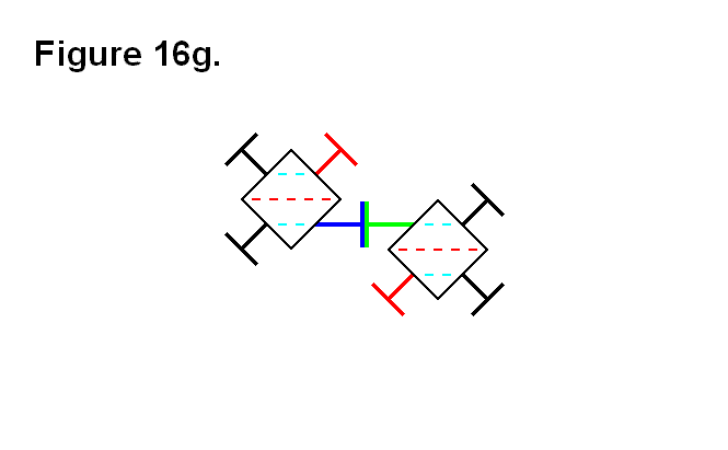
Finally, just as reversing the movement pattern halfway through the process of transferring module A from position row 1, column 2 to position row 1, column 3 could be used to accomplish that process in Figures 4a, 4b, and 4c, the same concept can also be applied to transferring module A from position row 1, column 3 to position row 2, column 4. Figure 4e shows the final result with module A in position row 2, column 4.

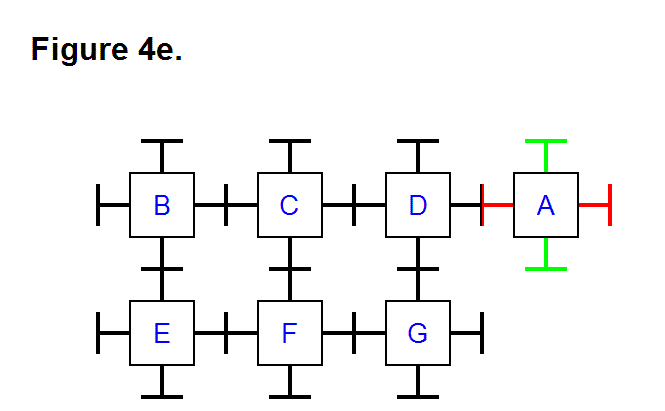
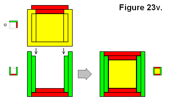
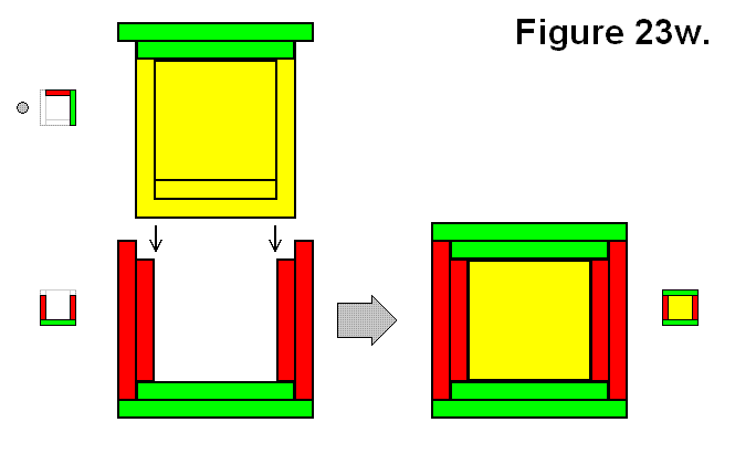
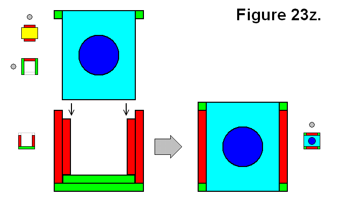
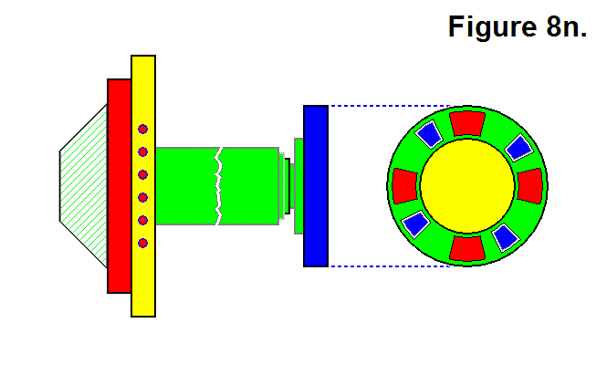
At this point it’s trivial to determine that module A can travel all the way around the rest of the matrix of modules B, C, D, E, F, and G, back to its initial position, by repeatedly applying the basic techniques of transferring a module along a row from one column to another, as well as around corners. Transferring a module vertically from one row to another in the same column involves using the same technique as transferring a module from one column to another column in the same row. In general, any module can be positioned to any other location to reshape either a 2-dimensional or 3-dimensional matrix consisting of any number of modules into any combination of connected patterns. Figure 4b shows how the modules in a matrix are not limited to being connected in a rectangular cycle arrangment (e.g., the way modules B, C, E, and F form a cycle); they can also be connected in a triangular cycle arrangement (e.g., the way modules A, C, and D form a cycle). Notice, also, that in Figure 4d modules A and D are connected together with two pairs of legs each; by using this feature it is possible to connect a series of several modules in this way, to double the tension strength. In a 3-dimensional matrix of modules, up to three pairs of legs can be connected between modules to triple the tension strength in a series of modules that are connected together in this way, since there are 6 legs for each module (instead of just 4 legs for each module as in a 2-dimensional matrix).

Determining the Distance Between the Centers of Two Cells Connected Together

DETERMINING THE DISTANCE BETWEEN THE CENTERS OF TWO CELLS CONNECTED TOGETHER

The geometric structural topology of a full cell consists of it having the following fundamental characteristics:

  1. the distance between the center of a cell and the point at which each leg pivots is a constant value
  2. for each cube face, the distances between the center of a cell and the point at which each leg pivots are all equal to each other
  3. for each cube face, the line segment between the center of a cell and the point at which each leg pivots is perpendicular to the line segments corresponding to each of the four adjacent cube faces

Many other characteristics about the topology of a cell can be derived from these fundamental characteristics and geometry. An essential key for a mesh of cells to form into objects is knowing its fundamental geometric structural topology and the distance between the centers of two cells connected together; this can be derived given that the following information is known about the modules in each cell that connect the two cells together:

  1. the length of the telescoping leg (this value is a variable within a fixed range)
  2. the angle a leg is pivoted, given as a value from a position perpendicular to the face of the cube; the absolute value of the angle a leg is pivoted will not be more than somewhere in the vicinity of 60 degrees
  3. either the actual connecting plate relative angle of rotation or the virtual connecting plate relative angle of rotation (i.e., derived from the effect of pivoting a leg about both of its cube face-oriented pivoting axes)

Figure 20a shows two cells connected together using a similar illustration convention as shown in Figure 12a from the article Geometrical Cell Dimension Limits and Requirements.

Figure 20b shows the same two cells connected together from Figure 20a including some 2-dimensional cartesian axes, labels for certain points, and labels for distance between these points. For the cartesian axes, the y, y’, and y” (from here on a dimension shall be generalized in the form w(n)) axes are all parallel and aligned along the y-dimension origin; the x(n) (for a 3rd dimension, shown in Figure 20e) and z(n) axes are all parallel to their corresponding dimensions. The legs that connect two cells together are always parallel and aligned about their axes; in Figure 20b they are aligned parallel to the y(n) axes and with the z(n) axes origins. The z’-axis is aligned to be centered at point C. The z-axis and z”-axis are arranged to be placed in alignment with the leg pivoting points B and D, respectively. In this case, both legs have pivot angle values of 0. Points A and E are the centers of their corresponding cells. Points B and D are the points at which each corresponding leg pivots. Point C is the center of the two connecting plates that are connected together. The distance between points A and B is the constant value a, which is equal to the distance between points D and E; this value corresponds to the distance described by the first list shown above, the fundamental geometric structural topology characteristics. The length of the telescoping leg from the left cell is b, which is the distance between the points B and C. The length of the telescoping leg from the right cell is c, which is the distance between the points Cand D. These leg lengths correspond to the first piece of information from the second list shown above.

In this case, determining the distance r between the centers of each cell is straighforward:

  (Formula #1)

In Figure 20c, the labelled points and corresponding distance labels of Figure 20b are shown without the cell body diagram illustrations and with one of the legs pivoted an angular value of α.

In this case the distance r between the centers of each cell is computed using the following equations and formula:

  (Formula #1a)
  (Formula #1b)
  (Formula #2)

In Figure 20d, both legs are pivoted about parallel normal vectors, meaning all the labelled points (A, B, C, D, and E) lie on the same plane, thus only a 2-dimensional diagram is necessary for analysis; the second leg is pivoted with an angular value of β.

For this situation, calculating the distance r between the centers of each cell needs to be computed using the following equations and formula (Equation # 2b was plugged in) by either changing the definition of the angles to take a polar coordinate format about their corresponding origins, instead of being an absolute value format, or switching from plugging in Equation # 2b to plugging in Equation # 2c into Formula # 3 when the centers of the cells are on opposite sides of the z(n) axes from each other.

  (Formula #2a)
  (Formula #2b)
  (Formula #2c)
  (Formula #3)

In Figure 20e, not only are both legs pivoted about the y(n) axes, but also not all the labelled points (ABCD, and E) have to lie on the same plane, thus a 3-dimensional diagram is necessary for analysis. The difference between Figure 20d and Figure 20e can be interpreted as a result of at least one of two reason:

  1. Connecting plate rotation took place between the two connecting plates connecting the cells together (at point C).
  2. Pivoting of one of the legs connecting the two cells together about the x(n)-y(n) plane took place.

The actual connecting plate relative angle of rotation or the virtual connecting plate relative angle of rotation (i.e., produced as a result of pivoting the legs) is the angular value f.

The following equations and formula are used to calculate the distance r between the centers of each cell for the case of Figure 20e. In this format the x(n)-component of the point A (the center of the cell on the left) is held fixed equal to 0. If necessary, as an intermediate step the modules can use the equations to derive calculated values and then re-apply those values to the formula using the same equations for calculating the distance r; this occurs when the pivot of the leg for the cell on the left is actually the resultant of the leg pivoting on both axes, when none of the legs on the faces adjacent to the legs connecting the cells together lie on the same plane, or when there is both leg pivoting and plate rotation. This principle is true for the apparent discrete cases of Figure 20d where all the labelled points (ABCD, and E) happen to lie on the same plane; all that is necessary for this situation is to utilize the 3-dimensional approach for Figure 20e. It is not necessary to be concerned about whether or not the centers of the cells are on opposite sides of the z(n) axes from each other, as it was for the case of Figure 20d, because this is resolved by having equations for all 3 dimensions.

  (Formula #3a)
  (Formula #3b)
  (Formula #3c)
  (Formula #4)

In general, only Formula # 4 is needed to calculate r for all cases. By knowing the geometric structural topology of the cells, and for every cell the angle values α, β, f, the values for lengths a, b, c, and the distance between the centers of any two two cells r, a mesh of cells has all the information about cell positions and states that it needs for knowing the state of its structure, and it has the geometric information that is necessary for changing its shape.

Sensor-Based Distance Determination for Centers of Two Cells Chained Through a Third Cell

SENSOR-BASED DISTANCE DETERMINATION FOR CENTERS OF TWO CELLS CHAINED THROUGH A THIRD CELL

Certain lengths and angles can either be measured with sensors or are known constants that can be used to calculate the distance between the centers of two cells connected to a middle (third) cell such that they are chained in series. In order to determine the distance, each involved module within each cell would have to perform calculations on shared readings from both its own sensors and sensors on the other modules that are involved. In Figures 22a and 22b, 3 cells A, B, and C are drawn as three-dimensional green wire frames to represent the core of the cells (i.e., the cube-shaped region that doesn’t include the telescoping legs and connecting plates). The red numbered lines represent the measureable sections, they are either the distance from the center of the cell cube to the center of the face on the cube surface (all are equal and constant), or the length of the telescoping leg (each one is a variable value). There are two ways that 3 cells can be chained in series. One is shown in Figure 22a, where two cells (A & C) are connected to the middle cell (B) on opposite sides through it along the y-axis. In either case, the numbered red lines are:

  1. Cell cube center to center of face for cell A connected to 2
  2. Leg of cell A connected to 1 and 3
  3. Leg of cell B connected to 4 and 2
  4. Cell cube center to center of face for cell B connected to 3 and 5
  5. Cell cube center to center of face for cell B connected to 4 and 6
  6. Leg of cell B connected to 5 and 7
  7. Leg of cell C connected to 6 and 8
  8. Cell cube center to center of face for cell C connected to 7

The lengths of the “cell cube center to center of face” sections are all equal to each other in length L (i.e., L1 = L4 = L5 = L8 = L). For simplicity, all angle values written in formulas in this articleare limited to a single-cycle range of angle (0 ≤ angle < 2π).
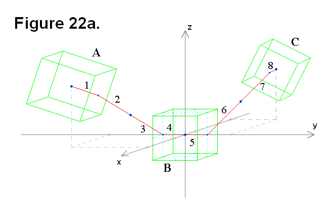
The other is shown in Figure 22b, where two cells (A & C) are connected to the middle cell (B) on adjacent sides through it along the positive y-axis, positive z-axis, and the x-y-z axes origin (where the 3 axes intersect).

In Figure 22c, the focus is on only some of the red lines, sections 1, 2, and 3 (or alternatively, sections 6, 7, and 8), in Figures 22a and 22b. Vector r1 (line segment OA) corresponds to sections 2 and 3 in Figures 22a and 22b, and vector r2 (line segment AC) corresponds to section 1 in Figures 22a and 22b. Points C1 and C2 are actually two possible graphical representations of a single point C, which is the center of the cell cube. The actual sensors are the universal joint horizontal and vertical angles, the connecting plate rotation angle, and the telescoping leg length. Readings from these sensors can be used as input values in conversion formulas as part of the process to perform the distance calculations. Since θ corresponds to the pivot angle of the leg, and the leg pivots on the face of the cell cube, it is never going to be more than a magnitude of 90° (i.e., 0 ≤ |θ| ≤ π/2).

The following equations written in terms of r are 3-dimensional vector and magnitude formulas:

   (Formula #1)
    (Formula #2)

Although r1 = L, r1 will remain in the equations for clarity. From Figure 22c, the following equations can be derived:

  (Equation # 1)
  (Equation # 2)
  (Equation # 3)
  (Equation # 4)
  (Equation # 5)

If  1 = 0 and  2 = 0, the following equations can be derived and used.

  (Equation # 6)
  (Equation # 7)
  (Equation # 8)
  (Equation # 9)
  (Equation # 10)

The following two equations are independent of any angle value 2.

  (Equation # 11)
  (Equation # 12)

The length of r0 can be calculated without θ1, using only r1, r2, and θ2, but ry and rz cannot.

  (Equation # 13)

The following two equations apply only to point C1, not C2.

  (Equation # 14)
  (Equation # 15)

To make it easier to analyze the diagram in Figure 22c, some of the sections are redrawn in Figure 22d (Cartesian diagram on left side). The separate red-green-blue triangle in Figure 22d on the right side is a diagram of vector OB perpendicular to the plane of the diagram for arbitrary values of  2. 

From Figure 22d, the following equations, which are independent of  2, can be derived:

  (Equation # 16)

If  1 = 0, the following equation can be derived.

  (Equation # 17)

For any angle value 2, in the y-z plane:

  (Equation # 18)
  (Equation # 19)
  (Equation # 20)

In red-blue-green triangle figure:

  (Equation # 21)
  (Equation # 22)

For  1 = 0 and arbitrary values of  2:

  (Equation # 23)

To generalize, the ρ-variables in the following equations are fixed to the formulas.

  (Equation # 24)
  (Equation # 25)
  (Equation # 26)

For any value of 1, Figure 20e shows the necessary components for continuing the geometric analysis to derive the necessary formulas. The Cartesian diagrams with the green wire frames are based on Figure 22c for representing arbitrary values of 1 and 2. The blue triangle involves lengths ρz and ρx, and introduces angle β to cover the situation of 1 = 0 and arbitrary values of 2. For 1 = 0, angle β is basically a function of 2 to allow for calculating α as a function of angles 1 and β; all that is necessary is to add the two angles.
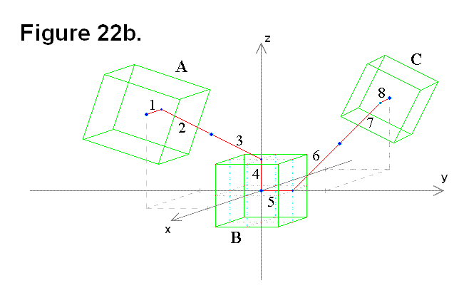
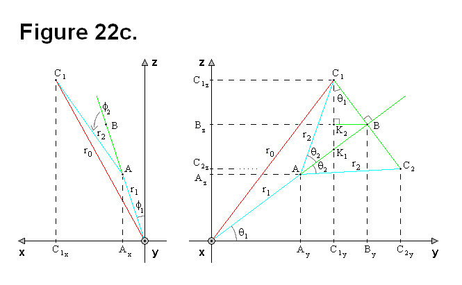
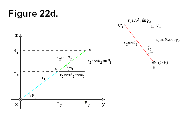
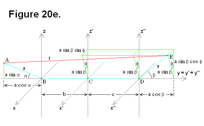
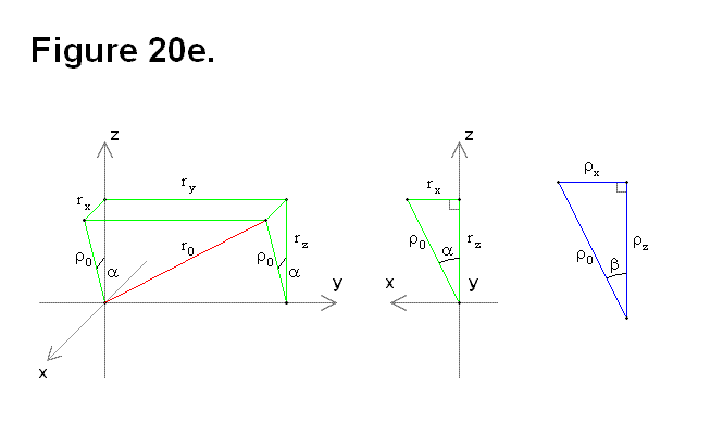
Based on Figure 22e, the following equations can be derived:

  (Equation # 27)
(Equation # 28)
  (Equation # 29)
  (Equation # 30)
  (Equation # 31)
  (Equation # 32)
  (Equation # 33)

Now from the previous equations, the following formulas can be derived:

  (Equation # 34)
  (Equation # 35)
  (Equation # 36)
  (Equation # 37)

To calculate the distance d from the origin O to the center of cell A (shown in Figure 22a), all that is necessary is to include section 4 in the equations:

  (Equation # 38)
  (Equation # 39)
  (Equation # 40)

The previous three equations are re-written to include both sections 1-4 and 5-8 in Figure 22a. The next three are for sections 1-4:

  (Equation # 41)
  (Equation # 42)
  (Equation # 43)

The next three equations are for sections 5-8:

  (Equation # 44)
  (Equation # 45)
  (Equation # 46)

The following equations result from adding the last six equations together, to get the formulas for the distance D from the center of cell A to the center of cell C in Figure 22a:

  (Equation # 47)
  (Equation # 48)
  (Equation # 49)

The following three equations represent sections 5-8 in Figure 22b:

  (Equation # 50)
  (Equation # 51)
  (Equation # 52)

Cell Structure Forming Pattern Possibilities

CELL STRUCTURE FORMING PATTERN POSSIBILITIES

There are several ways a module can be attached to other modules to form a partial cell, full cell, or inverse cell. In Figure 23a, the different side views of a single module is shown in various colors. The leg and connecting plate assembly is a darker blue, and the rest of the module is a different color for the type of side. For the opposite sides that are symmetric, the longer (lengthwise) side are green, and the shorter (widthwise) sides are red. The surface on which the leg mounts is light blue, and the opposite side is yellow. In this diagram, the truncated pyramid-shaped surface shown in this article: Module Connection Arrangement Patterns of a Cell is omitted, but the yellow side corresponds to the side on which it is mounted.

One type of connection of a module is to another single module via the connecting plates. This is shown in Figure 23b and is referred to as an “inverse cell.” The idea is that in the same way a mesh or matrix can be made of cells, and cells are made using modules, a mesh or matrix can also be made of inverse cells, and inverse cells can also be made using modules. In this figure, different colors do not necessarily signify different modules. Both the legs and the connecting plates of both modules are dark blue. On the left side of the line indicated by a vertical series of gray dashes is one module with a green lengthwise side shown, and on the right the other module with a red widthwise side shown. It is not necessary for the opposite types of side indicated by red or green to be aligned with each other from the two modules or to be aligned in general. It is only shown this way to make it easier to identify each module. The different resulting patterns will be categorized with abstract codes as connection types. A single module will be categorized simply as M. The resulting module structure in Figure 23b will be categorized as connection type T.

An expression describing the connection will also be given in the forms F → R or R ← F, meaning “F can form R,” where R is the resulting form and F is an abstract representation of “X + Y,” which means the joining of object X to object Y, and it is commutative (i.e., X + Y and Y + X are interchangeable). The objects X and Y each can be either a module M or a partially constructed cell R.

Expression: M + M → T

Another type of connection of a module M to another single module M is via the rectangular bases, which is to connect one along one of the green surfaces side (not shown) to the yellow widthwise side (not shown) of another in the type of orientation and alignment shown in Figure 23c. The smaller square to the right is an abstract icon representing the view angle of the figure with corresponding color pattern (shown for future reference). In this figure as well, different colors do not necessarily signify different modules. Both the legs and the connecting plates of both modules are dark blue. In this case it is necessary for the opposite types of side indicated by red or green to be aligned with each other from the two modules to be aligned. The different resulting patterns will be categorized with abstract codes as connection types. A single module will be categorized simply as M. The resulting module structure in Figure 23c will be categorized as connection type A. A formula describing the connection will also be given, for instance:

Expression: M + M → A

In the remaining part of this article the side views of the dark blue leg and connecting plate will be omitted from the diagrams and will only be limited to connections via the rectangular bases.

A single module can also be connected to a group made up of 2 to 5 modules connected together via their rectangular bases. Figure 23d shows one way of connecting a module M to each of a pair of modules A resulting in a partial cell in which all three modules share a common corner. The icon on the left is shown as a different angle than the figure image, and sometimes the view of the module in the back is obstructed by the one in front, so the gray circle with the smaller icons represent the side of the viewing direction of the figure (not present if viewing directions are the same) to reveal the presence of modules in the back on the icon. This resulting module structure will be categorized as connection type Bx.

Expression: A + M → Bx

Figure 23e shows a reflective way a of connecting a module M to each of a pair of modules A resulting in a partial cell in which all three modules share a common corner, which is a mirror image of the version in Figure 23d. This resulting module structure will be categorized as connection type By.

Expression: A + M → By

Instead of adding a single module M to a pair of modules resulting in a common corner, it can be added to one of the modules to be on the opposite side of the other module of an A structure. Figure 23f shows one version of this type of structure, categorized as connection type Ux.

Expression: A + M → Ux

Figure 23g shows another version of the type of structure similar in arrangement pattern to the structure of Figure 23f using an M and A structure, categorized as connection type Uy. These two from Figures 23f and 23g are opposites to each other in that they can join together to form a full cell.

Expression: A + M → Uy

Another way in which a single module M can be connected to a group of multiple modules connected together via their rectangular bases is shown in Figure 23h, which is to connect it to a set of 3 modules in a Ux structure. This is one version that results in this pattern where the 4 modules joined together results in a 2D alternating cycled pattern, to be categorized as connection type O.

Expression: Ux + M → O

The other way to join a single module M to 3 other modules to result in connection type O is shown in Figure 23i, by using a Uystructure.

Expression: Uy + M → O

Another way to connect a module M to a set of 3 modules in a Ux structure is shown in Figure 23j. This is one version that results in a pattern where the 4 modules joined together do not result in the 2D alternating cycled patterns of Figures 23h and 23i, to be categorized as connection type G.

Expression: Ux + M → G

Figure 23k also shows another way to connect a module M to a set of 3 modules, which are in a Uy structure, resulting in a G structure.

Expression: Uy + M → G

Another way in which a single module M can be connected to a group of multiple modules connected together via their rectangular bases is shown in Figure 23m, which is to connect it to a set of 4 modules in a G structure. This one is to be categorized as connection type Q.

Expression: G + M → Q

Figure 23n also shows another way to connect a module M to a set of 4 modules in a G structure which also results in a connection type Q.

Expression: G + M → Q

Figure 23o shows a way to connect a module M to a set of 4 modules in an O structure pattern for form a Q structure.

Expression: O + M → Q

Figure 23p shows a full cell, categorized as connection type C, made by connecting a module M to a Q structure.

Expression: Q + M → C

Forming a structure is not limited to being possible by adding just a module M to another structure. Two structures A and A can be joined together to form a structure. A structure O made by joining two structures A and A is shown in Figure 23q.

Expression: A + A → O

A structure G can be made by joining two structures A and A as shown in different perspectives in Figures 23r and 23s. Since it might not be simple to determine that different views are the same structure forming connection pattern, the modules are labeled A, B, C, and D to indicate which ones in Figure 23r can correspond to the ones in Figures 23s.

Expression: A + A → G


A structure Q can be made by joining two structures A and By as shown in Figure 23t.

Expression: A + By → Q

A structure Q can also be made by joining two structures A and Bx as shown in Figure 23u.

Expression: A + Bx → Q

A full cell structure Q can be made by joining two structures A and Ux as shown in Figure 23v.

Expression: A + Ux → Q

A full cell structure Q can also be made by joining two structures A and Uy as shown in Figure 23w.

Expression: A + Uy → Q

A full cell structure C can be made by joining two structures A and G as shown in Figure 23x.

Expression: A + G → C

A full cell structure C can also be made by joining two symmetrically opposite B structures Bx and By as shown in Figure 23y.

Expression: Bx + By → C

A full cell structure C can also be made by joining two symmetrically inverse U structures Ux and Uy as shown in Figure 23z.

Expression: Ux + Uy → C

The following table summarizes the expressions, and groups each connection F with matching results R or vice versa by separating each possible type of joining connection or result by a “|” symbol (meaning “or”), listed by number of modules in the resulting cell. If the subscript is omitted it means all versions are included.


Number of Modules Expression
2 M  + M   → A  | T
3 A  + M   → B  | U
4 O  | G   ← U + M  | A + A
5  Q   ← G + M  | O + M  | A + B  | A + U
6  C   ← Q + M  | A + G  | Bx + By  | Ux + Uy


The following table summarizes the distinct possible “|” separated R result patterns arranged in order of number of modules in each joining part.


Structure Connections Resulting Pattern Possibilities Notes
1: + 1 = 2 A  | T only one possible way to form each
+ 2 = 3 Bx  | By  | Ux  | Uy only one possible way to form each
+ 3 = 4 O  | G two symmetrically complementary possible ways to form each
+ 4 = 5 Q three possible ways to form, two are complementary to each other
+ 5 = 6 C only one possible way to form
2: + 2 = 4 O  | G only one possible way to form each
+ 3 = 5 Q four possible ways to form, 2 pairs of symmetrical compements
+ 4 = 6 C only one possible way to form
3: + 3 = 6 C two symmetrically complementary possible ways to form


Structure of a Sub-Module

STRUCTURE OF A SUB-MODULE

The Sub-Modules are assemblies that connect together to form Macro-Modules, and these Macro-Modules then connect to each other to form application structures. These Sub-Modules are all identical to each other in all aspects of structure (e.g., mechanically, electronically, operationally). They consist of two different types of bases and a leg. One of the bases is a Core Base Assembly (the “core” being the “nucleus” of the Macro-Module) and the other is the Connecting Plate Assembly. The Core Base Assembly is linked to the Connecting Plate Assembly by a Leg Assembly that can extend and retract. The Core Base Assembly can pivot the Leg Assembly about both axes which are perpendicular to the axis of the Leg Assembly (i.e., it can pivot in any direction just as an arm can pivot being mounted on the shoulder). The Connecting Plate Assembly can rotate in either clockwise or counter-clockwise directions about the axis of the leg. There are two ways the Sub-Modules can connect to each other. One involves the Core Base Assembly; this means of connecting involves connecting each one directly to four others and indirectly to a fifth one to form into a Macro-Module. The other involves the Connecting Plate Assembly; the Macro-Modules connect to each other by using this as a means for connecting together. The Core Base Assemblies can encase a Power Cell that can optionally be present or absent. The Sub-Modules can transmit and receive power and communication signals. If a Macro-Module doesn’t contain a Power Cell then it must utilize adjacent modules to acquire energy.

Figure 8a, below shows 3 views of the Core Base Assembly. It consists geometrically of two rectangular boxes and a square Truncated Pyramid with sides that slope at 45° angles. The rectangular boxes are of the same thickness, but one, shown as the External Block Region in the figure, has a perimeter that is larger than the other, shown as the Internal Block Region in the figure, of a thickness equal to their box thicknesses (the thickness that each rectangular box has in common with each other of being equal in length on those sides). The two rectangular boxes join together such that their centers are aligned and the box thickness perimeter of the larger rectangle circumscribes the smaller rectangle. The pyramid is of a size such that the edges of two opposite sides of the larger end of the pyramid meet flush with the smaller rectangle and have a space on the other two opposite sides that form space on either side of the surface of the smaller rectangle that are also equal in thickness to the box thicknesses of the rectangle shapes. The smaller end of the pyramid is a Connecting Plane for a cube-shaped Power Cell, also shown in the figure. This shape is necessary to allow the Sub-Modules to connect together in a specific pattern. The larger rectangle houses Connecting Points, which consist of pins and holes that are used to bond the Core Base Assemblies together. The Inward Side view is a view of the side that goes into the core of the Macro-Module.


Figure 8b, shown below, also shows 3 views of the Core Base Assembly, except that one of them is an Outward Side view. The Core Base Assembly actually consists of 2 moving parts, an Outer Sub-Module Assembly and an Inner Sub-Module Assembly. This Inner Sub-Module Assembly houses actuators and acts as a universal joint between the Outer Sub-Module Assembly and Leg Assembly that gives it the ability to pivot about both axes. The Perimeter of the Inner Sub-Module Assembly is shown within the Outward Side view of the Core Base Assembly shaded in blue; the rest of the view and the other side views show the region of the Outer Sub-Module Assembly. The Pyramid Well is the region that can be seen behind the Inner Sub-Module Assembly in the Outward Side view, which is a view of the inside of the Truncated Pyramid.

Figure 8c, shown below, shows 4 Core Base Assemblies and a Power Cell aligned to geometrically join together. 

Figure 8d, shown below, shows the 4 Core Base Assemblies and Power Cell from Figure 8c geometrically joined together such that the 4 Core Base Assemblies encompass the Power Cell.

Figure 8e, shown below, shows 5 Core Base Assemblies connected together.

Figure 8f, shown below, shows a 3-dimensional view of 2 Core Base Assemblies geometrically joined together.

Figure 8g, shown below, shows a 3-dimensional view of 3 Core Base Assemblies connected together. Their geometric pattern, wherein they are sharing a common corner, mechanically bonds them together when the pin-and-hole system is engaged along the edges where another Sub-Module is present.

Figure 8h, shown below, shows the Inner Sub-Module Assembly contained within a wireframe outline of a transparent Outer Sub-Module Assembly. The Leg Space & Pivot Channel represents the perimeter of the space within the Inner Sub-Module Assembly in which the Leg Assembly is located and moves.

Figure 8i, shown below, shows a hypothetical end of part of the Leg Assembly contained within a wireframe outline of a transparent Inner Sub-Module Assembly. The Leg End Pivoting Range shows the space needed by the end of the Leg Assembly for pivoting.

Figure 8j, shown below, shows a hypothetical Leg Assembly of undetermined length. It also shows the Connecting Plate Perimeter in relation to the Leg Assembly; the Connecting Plate and the Leg Assembly have the same center axis of symmetry, and the Connecting Plate can rotate about this axis. The Leg Assembly basically consists of a series of hollow tubes to allow it to extend and retract.

Figure 8k, shown below, shows the Connecting Plate Surface of the Connecting Plate Assembly. The Connecting Plate Arc Cross Section is a “side view” diagram of the Connecting Plate Assembly’s surface. The Connecting Plate Outer Ring serves as the mounting surface for the hooks and houses the plungers. This hook and plunger system acts as an interlocking mechanism between the two plates. The Connecting Plate Center Circle hypothetically serves as a region where electromagnets and communication components are housed.

Figure 8m, shown below, shows how two Connecting Plates from different modules can connect together. States 1 through 6 show the Connecting Sequence of the two plates, and states 6 through 9 show the Disconnecting Sequence of the two plates. To connect, the red plate engages the blue plate by rotating to the left, as shown in sequences 1-5; in sequence 6 the plungers are extended out to lock the plates together. To disconnect, the plungers are retracted in, as shown in sequence 7, and the red plate disengages the blue plate by rotating to the right, as shown in sequences 8 and 9.

Figure 8n, shown below, shows a full Lengthwise Side view of a Sub-Module along with a Connecting Plate Surface view.

Leg Pivot Range Requirement

LEG PIVOT RANGE REQUIREMENT

In the following figures, all the dashed lines are parallel to each other. The dashed red lines indicate imaginary lines between the two opposite corners of the cube-shaped nucleus, and the dashed light-blue lines indicate imaginary lines connecting the centers of the face of the cube-shaped nucleus, where the legs connect to them to pivot. Figure 16a shows how two modules connected together with 2 pairs of legs need the flexibility of the legs to be able to pivot at least 45° to the face of the cube-shaped nucleus.

Figure 16b shows a circumstance where the legs need to be able to pivot more than 45° in order for the two cells to connect together; it is the situation where the legs need to be able to pivot the furthest, which is determined by the dashed red lines being aligned with light blue dashed lines. The actual angle value is determined by how close the two cells can be to each other, and how close the two cells can be to each other is determined by the length of the fully retracted telescoping shaft (the leg) plus the thickness of the connecting plate.

Figures 16c and 16d show one way (they’re both the same type of connection, one is an upside-down view of the other) for the two cells to connect together when they are in the positions of the cells in figure 16b. The closest the two cells can come to each other in this situation is a value that is proportional to the absolute value of the tangent function with the argument value of φ + 45°, where φ is the angle between the face of the cube and the leg that is less than 45°. The ideal leg pivot range angular limit orthogonal to the face of the cube to implement would be as close to around 60° as possible, because as the angle approaches 45° the distance approaches infinity (in an exponential growth-like rate); it is not necessary to go beyond a leg pivot angular limit of about 60°, because anything greater than that is an approximately linearly decreasing rate, and would require the unfeasible implementation of the legs (i.e., they would have to be extremely thin) and other components that would be affected.


Figures 16e shows the two cells from figure 16b connected together using both pairs of legs. This or the connection arrangements of figures 16c and 16d would be the choice for connecting the two cells together if the two red dashed lines from each cell are not going to extend, beyond the boundary indicated by the light-blue dashed line, to be any further apart from each other than this.

In figure 16f, the two cells from figure 16b are connected together in an alternative way to the way the cells are connected together in figures 16c and 16d. This connection arrangement would be the choice for connecting the two cells together if the two red dashed lines from each cell are going to extend, beyond the boundary indicated by the light-blue dashed line, to be any further apart from each other than this.

In figure 16g, the two cells are in positions where the two red dashed lines are farther apart, and the legs are back to being pivoted at 45° angles to the faces of the cube-shaped nuclei.

Leg Thickness Limits Based on Pivoting Ranges and Well Perimeter Edge

LEG THICKNESS LIMITS BASED ON PIVOTING RANGES AND WELL PERIMETER EDGE

The thickness of the outermost telescoping leg segment (the rectangular sides of a cross section) determines the leg’s pivoting range limit. For a thicker leg the pivoting range limit is smaller, and for a thinner leg the pivoting range limit is larger. The tradeoffs for a thicker leg include the following features:

  1. more strength against leg bending strain or damage
  2. more space for the mechanical system to telescope the leg
  3. more leg segments for telescoping the leg

For both Figures 21a and 21b the variable a and the module core assembly base component ratios are based on the calculations from the Optimal Ratio Calculation for Module Core Assembly Base Component article.Figure 21a is a diagram of a lengthwise cross section of the base of the module that forms the module core assembly base component as a black outline and a representation of the boundary of the leg that can enter the well as a blue line. The lengthwise well perimeter is indicated by the red vertical lines. The variable L represents half the lengthwise thickness of the leg, and the variable θL represents the lengthwise plane of rotation angle for the leg from a perpendicular position relative to the face of the cell cube.

The following equations and calculations are derived from the geometrical information provided by Figure 21a:

                           (Equation #1)
                                                                                   (Equation #2)
(Formula #1)
                                                      (Formula #2)

Figure 21b is a diagram of a widthwise cross section of the base of the module that forms the module core assembly base component as a black outline and a representation of the boundary of the leg that can enter the well as a blue line. The widthwise well perimeter is indicated by the red vertical lines. The variable W represents half the widthwise thickness of the leg, and the variable θW represents the widthwise plane of rotation angle for the leg from a perpendicular position relative to the face of the cell cube.

The following equations and calculations are derived from the geometrical information provided by Figure 21b:

                           (Equation #3)
                                                                                   (Equation #4)
(Formula #3)
                                                      (Formula #4)
Graph #1 Graph #2
Graph # 1 shows a plot of the angle versus the rectangular lenghwise thickness factor (to ratio variable a) of the leg. Green is for an angle of 45 degrees, and red is for an angle of 60 degrees. Beyond 60 degrees the decrease is almost linear.

Graph # 2 shows a plot of the angle versus the rectangular widthwise thickness factor (to ratio variable a) of the leg. Green is for an angle of 45 degrees, and red is for an angle of 60 degrees. Beyond 60 degrees the decrease is almost linear.

Graphs # 1 and # 2 were generated using the following Matlab code: matlab.txt

Figure 21c shows a view of the face of the module core assembly base component with the perimeter of the well as a blue rectangular line. The well perimeter and the surface plane of the face that it intersects with forms the well perimeter edge. The green rectangle represents the leg thickness and rectangular perimeter as a cross section of a leg that can pivot up to 45 degrees, and the red rectangle represents the leg thickness and rectangular perimeter as a cross section of a leg that can pivot up to 60 degrees.

In reality, the intermediate universal joint-like component between the module core assembly base component and the first segment of the leg will affect either the shape of the rectangle on the widthwise side of the leg or the shape of the well, because of the cylindrical twisting effect introduced by the universal joint-like component. Also, the universal joint-like component can also affect the lengthwise range, since it pivotally mounts to the module core assembly base component in the region the leg would enter in the well; this might be a limitation that can be minimized or eliminated with an appropriate design for the structure of this universal joint-like component.


Geometrical Cell Dimension Limits and Requirements

GEOMETRICAL CELL DIMENSION LIMITS AND REQUIREMENTS

In order to be able to achieve some of the needed features and capabilies, there are some minimum requirements in length ratios and pivot angles which can be calculated. There are also certain constraints in length ratios imposed by the geometric shapes of the modules. Figure 12a shows equivalences of module schematics, a basic more symbolic version on the left side, and a more detailed image of a cell on the right side. The image on the right side is the one that will be used as a template for the subject matter of this article. The connecting plates (a side view) are shaded in yellow; the black lines going from the connecting plates to the inner blue square in the center represent the telescoping shafts (the legs). The points where the legs connect to the blue square is where the legs pivot about both axes (in this 2-dimensional image we shall only consider pivoting about the axis that is perpendicular to the plane of the image). The green square represents the perimeter of the cell nucleus, and are also side views of the faces of the cell nucleus. The dashed lines will be used for reference measurements.

In Figure 12b the distance between points a (the center of the cell) and b (the point that intersects the surface of the connecting plate while the leg is completely retracted, and the leg axis) is equal to A; this line segment is shown as a green line.

Recalling Figure 7c from the article Diagonal Lattice Reconfiguration Using Leg Extending Capabilities, in order to make it possible for the leg from module A to be able to reach and connect to module C, it is necessary that the legs be able to extend a distance that is long enough to span the distance imposed by the three modules in the bottom row, having module B on the left side, where the row legs that are connected together are fully retracted.

This length of the extended leg associated with this minimum requirement length is represented in Figure 12c as the distance between points a (the center of the cell) and b’ (the point that intersects the surface of the connecting plate while the leg is extended to meet the minimum length requirement, and the leg axis) is equal to B; this line segment is shown as a green line.

An equation can now be formulated; in the top row of Figure 7c, the distance between module A and module C is 2B; in the bottom row (starting with module B) of Figure 7c, the distance between the center of the modules on either end would be 4A. These two values, 2B and 4A, are related in the following way: 2B > 4A; by simlifying this equation the following equation is derived:

 B > 2A       (Equation 1)

 In Figure 12d the leg axis component distance between points c (the corner of the nucleus perimeter) and d (the edge of the underside of the connecting plate while the leg is fully retracted) is equal to C; this corresponds to the distance between the face of the nucleus and the underside of the connecting plate while the leg is fully retracted.

When the leg pivots 45 degrees, as shown in Figure 12e, the connecting plate edge comes close to the corner of the nucleus cube; if length C is not long enough then the connecting plate will strike the nucleus if it attempts to pivot 45 degrees, which will prevent it from being able to achieve this. The red dashed line c’ represents the orthogonal limit plane imposed by the corner of the nucleus, and the red dashed line d’ represents the underside plane of the connecting plate when the leg is fully retracted; these two planes can approach each other, but they cannot be intersecting.

Recalling Figure 4d from the article Basic Module Transfers, Movements, and Connections, in order to make it possible for module A to be able to connect to module D with two adjacent legs from each module, not only it is necessary that the legs be able to pivot by at least 45 degrees, but it is also necessary that the radius of the connecting plates not reach a certain maximum limit

The distance between the center of the two connecting plates on the legs that are pivoted 45 degrees towards each other in Figure 12f is D (it is also equal to the line segment shown as a green line); based on this observation, the circumference of the connecting plate must be less than D, which means that the radius has to be less than D/2.

In Figure 12g the distance between points c (the corner of the nucleus) and a’ (the point that intersects the surface of the nucleus and the leg axis) is equal to E; this line segment is shown as a green line.

The length between the point where the leg pivots and the face of the nucleus along the axis of the leg is a/2 (see Optimal Ratio Calculation for Module Core Assembly Base Component); by using trigonometry, the following equation can be derived: D = √2(E-a/2). Solving for E produces the following equation:

E = (√2D + a)/2     (Equation 2)

This means that now we know that the radius of the connecting plate has to be less than √2(E-a/2)/2. With some trigonometry and geometric manipulations, and the fact that C has to result in the gap greater than zero between planes c’ and d’ in Figure 12e, the following equation can also be derived: 2C + a > D + √2a. By solving for C in this equation, the following equation can be derived:

C > (D+(√2-1)a)/2     (Equation 3)

If the thickness of the connecting plate along the leg axis is T, then the following equation relating length A to lengths C and Ecan be derived: A = C + E + T. By substituting for the values of C and E in this equation, the following equation can be derived: A < (D+(√2-1)a)/2 + (√2D + a)/2 + T; simplifying this equation produces:

A < ((√2 + 1)D + √2a)/2 + T     (Equation 4)


Pattern for Element Core Electronic Connections

PATTERN FOR ELEMENT CORE ELECTRONIC CONNECTIONS

The sub-modular entities in a basic level modular element need to be able to electronically connect to each other through their core bases, to transfer power or communicate with each other. In a full basic level modular element each entity can electronically connect directly to every other entity, except for the one on the opposite side, since they are adjacent to each other.

One way to make it possible for entities that are on opposite sides of each other to electronically connect is to provide a relay path through some of the adjacent entities; a relay channel needs to be present in every entity to accomplish this. Since the entities are uniformly manufactured, the relay paths can also be present in a uniform pattern.

There is a simple way to implement this solution; the figure below is a schematic diagram showing how the entities can electronically connect to both the adjacent and opposite side entities. The yellow box contains entity core base components labeled A, B, C, D, and E. Component A is the symbol for an electronic relay path through an entity for connecting two entities that are opposite from each other. Component B is an electronic connection between two entities; the clubbed ends indicate the entities they electronically connect by being encased in the symbol for an entity, component D. Component C is similar to component B, except the ends are X-shaped and it emphasizes that it is a relayed path for electronically connecting entities that are opposite from each other. The path symbolized in component B is only an electronic connection, not a representation of the path through space (i.e., it is not a mechanical schematic). Component E is the symbolic pattern of the uniformity of each entity (they are also symmetric in 180 degree rotations); each entity in the schematic diagram has an identical pattern to it, if rotated by 90 degrees when necessary.

Adjacent entities have one electronic connection, but entities that are at opposite sides of each other have two electronic connections; this is necessary since some element modules night not be full modules (meaning one of those paths is not present because the entity that has it is not present).


Optimal Ratio Calculation for Module Core Assembly Base Component

OPTIMAL RATIO CALCULATION FOR MODULE CORE ASSEMBLY BASE COMPONENT

Six assemblies, and an optional power cube, form a module; each assembly is made up of several distinct components: a telescoping leg, one base that connects directly to the telescoping leg (the connecting plate), a module core base, and an intermediate component that connects the telescoping leg to the module core base. To maximize the space for the intermediate component of the assembly that connects the telescoping leg to the assembly’s module core connector base, there are optimal ratios for the lengths of the sides of the part of the assembly that connects to 4 other assemblies and the power cell (the module core assembly base), to form a module, and they can be calculated. Figure 1, below, is a diagram that shows a widthwise cross section of this component of the assembly.

Optimization is accomplished by setting the length of line segment CP to line segment CT and line segment CH, which are all equal to length r. For this diagram, the following equations are derived or set:

√2s = r                                                         (Equation 1)
w = a + b + s     →     w – a = b + s            (Equation 2)
s + a/2 = b + 2a     →      s = b + 3a/2      (Equation 3)
CP = CT = CH = r                                        (Equation 4)
(a/2)2 + (b + s)2 = r2                                  (Equation 5)

he ratios can be boiled down to a specific ratio k between 2 lengths, a and w (a ∝ w → ka = w); to solve for the constant of proportionality k, solve for a and w:

Plug equation 3 into equation 2:

w – a = 2b + 3a/2     →     b = w/2 – 5a/4      (Equation 6)

Plug equation 3 into equation 1:

√2(b + 3a/2) = r      (Equation 7)

Plug equation 2 into equation 5:

(a/2)2 + (w – a)2 = r2      (Equation 8)

Plug equation 7 into equation 8:

(a/2)2 + (w – a)2 = 2(b + 3a/2)2      (Equation 9)

Plug equation 6 into equation 9:

(a/2)2 + (w – a)2 = 2((w/2 – 5a/4) + 3a/2)2 → 4w2 – 20aw + 9a2 = 0      (Equation 10)

Setting a = 1 and solving for w in equation 10:

w = (5 +/- 4)/2 = 0.5 and 4.5

Since w > a, w = 4.5; so, the ratio k between a and w is:

k = 4.5

Solving for b, r, and s (for a = 1):

b = (4.5)/2 – 5(1)/4 = 2.25 – 1.25 = 1
r = √2((1) + 3(1)/2) = √2∙2.5 ≈ 3.536
s = (1) + 3(1)/2 = 2.5

Figure 2, below, is a diagram that shows a lengthwise cross section of this component of the assembly.

For this diagram, the following equations is derived:

d = 2a + b + s     (Equation 11)

Solving for d (for a = 1):

d = 2(1) + (1) + 2.5 = 5.5

Ratio of each length in terms of a:

b = a                         (Formula #1)
w = 4.5∙a                         (Formula #2)
d = 5.5∙a                         (Formula #3)
r ≈ 3.536∙a                         (Formula #4)
s = 2.5∙a                         (Formula #5)